Introduction to Graph Theory - Part 7

Imagine you're organizing exam schedules at a university. Some students are enrolled in multiple courses, so those exams can't happen at the same time. How many time slots do you need to schedule all exams without conflicts? Or consider a map: you want to color each country so that neighboring countries have different colors. How many colors do you need?

These two questions look completely different, but they are both instances of the same graph theory problem: graph coloring. The idea is deceptively simple — assign colors to vertices so that no two adjacent vertices share the same color — yet it leads to some of the deepest and most celebrated results in mathematics.

Vertex Coloring

Let's start with the basic definition. Given a graph, we want to assign a color to each vertex such that no edge connects two vertices of the same color.

Definition 35. A proper coloring of a graph $G = (V, E)$ is a function $c: V \rightarrow \{1, 2, \ldots, k\}$ such that $c(u) \neq c(v)$ for every edge $(u, v) \in E$.

We use numbers to represent colors — $1$ might stand for red, $2$ for blue, and so on. The important thing is not which colors we use, but how many we need.

Definition 36. A graph $G$ is $k$-colorable if it admits a proper coloring using at most $k$ colors.

Definition 37. The chromatic number of a graph $G$, denoted $\chi(G)$, is the smallest $k$ such that $G$ is $k$-colorable.

The chromatic number captures the minimum number of colors we need. A graph with $\chi(G) = 3$, for instance, can be properly colored with three colors but not with two.

Chromatic Numbers of Familiar Graphs

Let's figure out the chromatic numbers of some graph classes we already know. This will build our intuition before we look at more general results.

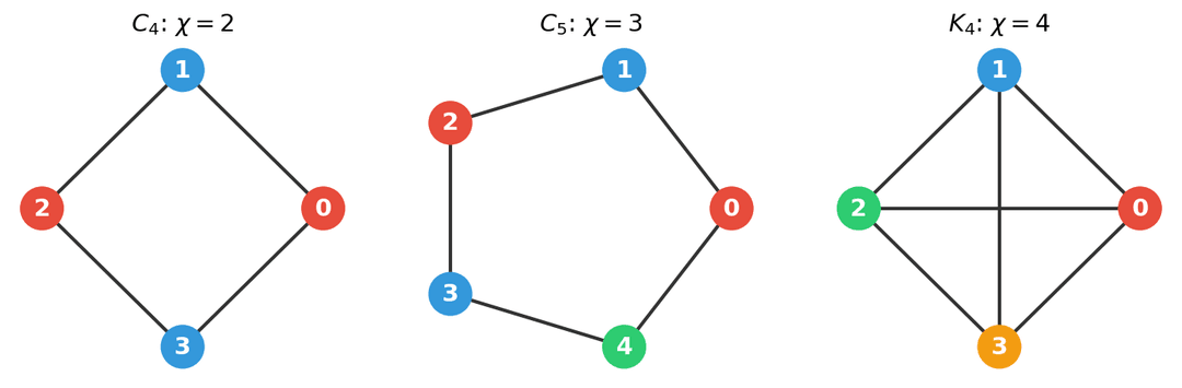
Complete graphs. In $K_n$, every vertex is adjacent to every other vertex. No two vertices can share a color, so we need a different color for each vertex. Therefore $\chi(K_n) = n$.

Bipartite graphs. A bipartite graph has two groups $A$ and $B$ with edges only between the groups. We can color all vertices in $A$ with color $1$ and all vertices in $B$ with color $2$. If the graph has at least one edge, we need both colors, so $\chi(G) = 2$. If it has no edges at all, one color suffices.

This observation actually gives us a useful characterization.

Observation 7. A graph with at least one edge is bipartite if and only if $\chi(G) = 2$.

Cycles. For even cycles $C_{2k}$, we can alternate two colors around the cycle: $1, 2, 1, 2, \ldots$, and the last vertex gets a different color from the first. So $\chi(C_{2k}) = 2$ — which makes sense, because even cycles are bipartite. For odd cycles $C_{2k+1}$, two colors don't work: when we try to alternate, the last vertex ends up adjacent to the first vertex with the same color. We need a third color, so $\chi(C_{2k+1}) = 3$.

Trees. Every tree with at least two vertices is bipartite — we can split the vertices into two groups based on their distance from any fixed vertex (even distance vs. odd distance). So $\chi(T) = 2$ for any tree with at least one edge.

The empty graph. A graph with no edges can be colored with a single color: $\chi(G) = 1$.

Greedy Coloring

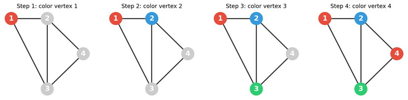
We've computed chromatic numbers for specific graph classes, but what about arbitrary graphs? There is a simple strategy that always produces a valid coloring: go through the vertices one by one and assign each vertex the smallest color that doesn't conflict with its already-colored neighbors. This is called greedy coloring.

More precisely, fix an ordering $v_1, v_2, \ldots, v_n$ of the vertices. For each vertex $v_i$, look at the colors assigned to its neighbors among $v_1, \ldots, v_{i-1}$ (the vertices already processed), and assign $v_i$ the smallest positive integer not used by any of those neighbors.

This procedure always produces a proper coloring — by construction, no two adjacent vertices receive the same color. The question is: how many colors does it use?

Observation 8. When coloring vertex $v_i$, at most $d(v_i)$ of its neighbors have already been colored. Since each of those neighbors uses one color, we need at most $d(v_i) + 1$ colors for $v_i$. Taking the maximum over all vertices gives us the following bound.

Theorem 6. For any graph $G$, the greedy algorithm uses at most $\Delta(G) + 1$ colors, where $\Delta(G)$ denotes the maximum degree of $G$. In particular, $\chi(G) \leq \Delta(G) + 1$.

This bound is easy to achieve — just run the greedy algorithm — and it's never too far off. But is it tight? For complete graphs, $\Delta(K_n) = n - 1$ and $\chi(K_n) = n = \Delta + 1$, so the bound is tight. For odd cycles, $\Delta(C_{2k+1}) = 2$ and $\chi(C_{2k+1}) = 3 = \Delta + 1$, so again the bound is tight.

But for most graphs, we can actually do better. The following classic theorem tells us that complete graphs and odd cycles are the only cases where the bound is tight.

Theorem 7 (Brooks, 1941). If $G$ is a connected graph that is neither a complete graph nor an odd cycle, then $\chi(G) \leq \Delta(G)$.

We won't prove Brooks' theorem here, but it is a powerful result: it tells us that except for two very specific graph families, the naive greedy bound can always be improved by one.

The Four Color Theorem

We started this article with map coloring, so let's return to it. When coloring a map so that neighboring countries have different colors, the underlying graph is planar — it can be drawn in the plane without any edges crossing¹.

For over a century, mathematicians asked: how many colors do you need to color any map? It was easy to show that five colors always suffice. But four? That question turned into one of the most famous problems in mathematics.

Theorem 8 (Appel and Haken, 1976). Every planar graph is $4$-colorable.

This is the Four Color Theorem. It states that no matter how complicated a map is, four colors are enough to color it so that no two neighboring countries share a color.

The history of this theorem is remarkable. It was first conjectured in 1852 by Francis Guthrie, a student who noticed that four colors seemed sufficient for coloring the counties of England. For over a hundred years, many mathematicians attempted proofs, and several "proofs" turned out to be incorrect.

The eventual proof by Kenneth Appel and Wolfgang Haken in 1976 was groundbreaking — and controversial. It was one of the first major theorems to rely on a computer: the proof reduced the problem to $1{,}936$ special configurations, each of which was verified by a computer program. Many mathematicians were uncomfortable with a proof that no human could check entirely by hand. Since then, the proof has been simplified and formally verified using proof assistants, putting the remaining doubts to rest².

To see that four colors are sometimes necessary, consider $K_4$: it is planar (you can draw it without crossings) and has $\chi(K_4) = 4$. So the bound of four is tight.

Edge Coloring

So far, we've been coloring vertices. But we can also color edges — and this turns out to be just as interesting.

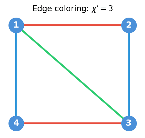
Definition 38. A proper edge coloring of a graph $G$ is an assignment of colors to edges such that no two edges sharing a vertex have the same color.

Definition 39. The chromatic index of a graph $G$, denoted $\chi'(G)$, is the smallest number of colors needed for a proper edge coloring.

Think of it this way: if the edges represent tasks and a shared vertex means two tasks conflict (they need the same resource), then the chromatic index tells us the minimum number of rounds needed to complete all tasks without conflicts.

How many colors do we need? At any vertex $v$, all edges touching $v$ must receive different colors, so we need at least $\Delta(G)$ colors. The following theorem tells us that this lower bound is nearly tight.

Theorem 9 (Vizing, 1964). For any graph $G$, we have $\Delta(G) \leq \chi'(G) \leq \Delta(G) + 1$.

Vizing's theorem is elegant in its simplicity: the chromatic index is always either $\Delta(G)$ or $\Delta(G) + 1$ — there are no other possibilities. Graphs where $\chi'(G) = \Delta(G)$ are called class 1, and those where $\chi'(G) = \Delta(G) + 1$ are called class 2. Determining which class a graph belongs to is, in general, an NP-complete problem.

Applications

Graph coloring is far more than a theoretical curiosity. Let's return to the exam scheduling problem from the introduction. We create a graph where each course is a vertex and two courses are connected by an edge if they share a student. A proper coloring then assigns time slots to exams so that no student has two exams at the same time, and the chromatic number tells us the minimum number of time slots needed.

Other applications follow the same pattern. In register allocation during compilation, variables that are used at the same time cannot share a CPU register — color the interference graph, and each color corresponds to a register. In frequency assignment for wireless networks, nearby transmitters that share a frequency will interfere — color the conflict graph, and each color is a frequency channel. In all these cases, the structure of the graph captures the conflicts, and the chromatic number captures the minimum resources needed to resolve them.

Looking Ahead

Graph coloring showed us that simple questions about graphs can lead to deep mathematics and famous open problems. In the next and final part of this introduction, we will explore matchings — the problem of pairing up vertices through edges so that no vertex is left doubly matched. This connects beautifully to both bipartite graphs and the algorithmic side of graph theory.