Network Flows - Part 6

In the previous parts, we focused on pushing as much flow as possible from source to sink. But in many real-world scenarios, not all routes are created equal. Shipping goods through one city might be cheap, while routing them through another might be expensive. When we care about both how much we send and what it costs, we need the minimum-cost flow problem — a beautiful generalization that ties together maximum flow, shortest paths, and linear programming.

The Problem

Let's extend our flow networks with a new ingredient: a cost for each arc.

Definition 12. A minimum-cost flow network is a tuple $N = (D, s, t, c, w)$, where $(D, s, t, c)$ is a flow network as before, and $w: A \rightarrow \mathbb{R}$ is a cost function assigning a cost $w(a)$ to each arc $a \in A$. The cost $w(a)$ represents the cost per unit of flow on arc $a$.

Definition 13. The cost of a flow $f$ is $\text{cost}(f) = \sum_{a \in A} w(a) \cdot f(a)$.

Now we can state the problem precisely.

Minimum-Cost Maximum Flow Problem. Given a minimum-cost flow network $N = (D, s, t, c, w)$, find a maximum flow $f$ that minimizes $\text{cost}(f)$ among all maximum flows.

Think of the supply chain from Part 1: we want to transport as much product as possible (maximum flow), but among all ways of doing so, we want the cheapest one (minimum cost). The two objectives are lexicographic — first maximize flow, then minimize cost.

There is also a more general formulation where we fix a desired flow value $d$ and ask for the cheapest flow of value exactly $d$. The maximum-flow version is the special case where $d = |f^*|$.

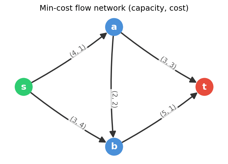
Let's set up a running example. Consider the network with vertices $\{s, a, b, t\}$, arcs and capacities $c(s,a) = 4$, $c(s,b) = 3$, $c(a,b) = 2$, $c(a,t) = 3$, $c(b,t) = 5$, and costs $w(s,a) = 1$, $w(s,b) = 4$, $w(a,b) = 2$, $w(a,t) = 3$, $w(b,t) = 1$.

The cheapest route from $s$ to $t$ goes through $a$ and then directly to $t$ (cost $1 + 3 = 4$ per unit), while the route through $b$ costs more per unit ($4 + 1 = 5$) but has more capacity. The challenge is finding the right balance.

Residual Costs

In Part 3, we introduced the residual graph to capture where more flow can be sent. For minimum-cost flows, we need to extend the residual graph with costs.

Definition 14. Given a flow $f$ in a minimum-cost flow network, the residual cost of an arc in the residual graph $D_f$ is defined as:

• For a forward arc $(u,v)$: $w_f(u,v) = w(u,v)$. Sending more flow along this arc costs $w(u,v)$ per unit.
• For a backward arc $(v,u)$: $w_f(v,u) = -w(u,v)$. Cancelling flow on $(u,v)$ saves $w(u,v)$ per unit, so the residual cost is negative.

The backward arc costs are the key insight. When we "undo" flow on an arc, we recover the cost we previously paid. This means that a negative-cost cycle in the residual graph represents a way to reroute existing flow to reduce the total cost without changing the flow value — we push flow around the cycle, and the negative total cost means we save money.

Negative Cycle Optimality

This observation leads to a clean characterization of optimal flows.

Theorem 8 (Negative Cycle Optimality). A feasible flow $f$ of a given value is minimum-cost if and only if the residual graph $D_f$ contains no negative-cost directed cycle.

Proof. For the "only if" direction: suppose $D_f$ contains a directed cycle $C$ with negative total cost $w_f(C) = \sum_{(u,v) \in C} w_f(u,v) < 0$. Let $\delta = \min_{(u,v) \in C} c_f(u,v) > 0$ be the minimum residual capacity along $C$. We can push $\delta$ units of flow around $C$. Since $C$ is a cycle, the flow value doesn't change (whatever enters a vertex also leaves it), but the cost decreases by $\delta \cdot |w_f(C)| > 0$. So $f$ was not minimum-cost.

For the "if" direction, the argument is more involved and relies on linear programming duality. The idea is that if no negative-cost cycle exists, we can construct a set of vertex potentials (dual variables) that certify optimality via complementary slackness¹. We omit the full proof here.

The Cycle-Canceling Algorithm

The negative cycle optimality condition immediately suggests an algorithm: start with any maximum flow and repeatedly cancel negative-cost cycles until none remain.

Cycle-Canceling Algorithm:

1. Find a maximum flow $f$ (using Edmonds-Karp or any max-flow algorithm).
2. Build the residual graph $D_f$ with residual costs.
3. Search for a negative-cost directed cycle $C$ in $D_f$.
4. If no negative cycle exists, stop — $f$ is a minimum-cost maximum flow.
5. Otherwise, compute $\delta = \min_{(u,v) \in C} c_f(u,v)$ and push $\delta$ units around $C$.
6. Go to step 2.

Finding a negative cycle can be done using the Bellman-Ford algorithm, which detects negative cycles in $O(nm)$ time.

Observation 3. Each iteration of the cycle-canceling algorithm strictly decreases the cost of the flow while preserving the flow value.

For integer capacities and costs, the algorithm terminates because the cost is an integer that decreases by at least $1$ in each iteration and is bounded below. However, the number of iterations can be large — proportional to the total cost, which may be exponential in the input size. More sophisticated cycle selection rules (such as always canceling the minimum mean cost cycle) lead to polynomial-time variants, but we won't go into those details here.

The Successive Shortest Paths Algorithm

There is an alternative approach that builds the minimum-cost maximum flow from scratch, rather than first finding any maximum flow and then repairing it. The idea is simple: send flow along the cheapest possible route, one unit at a time.

Successive Shortest Paths Algorithm:

1. Initialize $f(a) = 0$ for every arc $a$.
2. Build the residual graph $D_f$ with residual costs.
3. Find a shortest path (minimum total cost) from $s$ to $t$ in $D_f$ using the residual costs as edge weights.
4. If no $s$-$t$-path exists, stop — $f$ is a minimum-cost maximum flow.
5. Otherwise, let $P$ be the shortest path and $\delta = \min_{(u,v) \in P} c_f(u,v)$.
6. Push $\delta$ units of flow along $P$ (same as in Ford-Fulkerson).
7. Go to step 2.

This algorithm augments flow along the cheapest augmenting path instead of the shortest (fewest arcs) augmenting path. Each augmentation simultaneously increases the flow value and ensures minimum cost for the current flow value.

Theorem 9. The successive shortest paths algorithm maintains the invariant that after each augmentation, the current flow is a minimum-cost flow among all flows of the same value.

Proof sketch. Initially, the zero flow is trivially minimum-cost (it's the only flow of value $0$). Suppose the current flow $f$ with value $|f|$ is minimum-cost. We augment along a shortest path $P$ in the residual graph. If the resulting flow $f'$ were not minimum-cost for value $|f'|$, there would be a cheaper flow $f''$ of the same value. The difference between $f'$ and $f''$ can be decomposed into cycles in the residual graph of $f'$. But the shortest-path augmentation guarantees that no negative-cost cycle exists in $D_{f'}$² — a contradiction.

There is one subtlety: the residual graph may contain negative-cost arcs (the backward arcs), so we cannot directly use Dijkstra's algorithm for the shortest-path computation. However, we can use Bellman-Ford ($O(nm)$ per iteration), or — more cleverly — maintain vertex potentials to transform all residual costs to non-negative values, enabling Dijkstra's algorithm ($O(m + n \log n)$ per iteration with a Fibonacci heap).

With integer capacities, each augmentation sends at least $1$ unit, so the algorithm performs at most $|f^*|$ augmentations. Using Bellman-Ford, the total running time is $O(nm \cdot |f^*|)$. With the potential-based Dijkstra approach, each iteration costs $O(m + n \log n)$, giving $O((m + n \log n) \cdot |f^*|)$.

A Worked Example

Let's trace the successive shortest paths algorithm on our running example: $c(s,a) = 4$, $c(s,b) = 3$, $c(a,b) = 2$, $c(a,t) = 3$, $c(b,t) = 5$, and costs $w(s,a) = 1$, $w(s,b) = 4$, $w(a,b) = 2$, $w(a,t) = 3$, $w(b,t) = 1$.

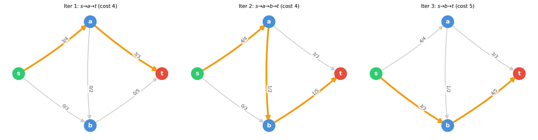
Iteration 1. We find the shortest (cheapest) path from $s$ to $t$. The candidates:

• $s \to a \to t$: cost $1 + 3 = 4$, bottleneck $\min(4, 3) = 3$.
• $s \to a \to b \to t$: cost $1 + 2 + 1 = 4$, bottleneck $\min(4, 2, 5) = 2$.
• $s \to b \to t$: cost $4 + 1 = 5$, bottleneck $\min(3, 5) = 3$.

Both $s \to a \to t$ and $s \to a \to b \to t$ have cost $4$. Let's pick $s \to a \to t$ with bottleneck $3$. We push $3$ units: $f(s,a) = 3$, $f(a,t) = 3$. Flow value: $3$. Cost: $3 \cdot 1 + 3 \cdot 3 = 12$.

Iteration 2. Residual graph: forward arcs $(s,a)$ with capacity $1$ and cost $1$, $(s,b)$ with capacity $3$ and cost $4$, $(a,b)$ with capacity $2$ and cost $2$, $(b,t)$ with capacity $5$ and cost $1$; backward arcs $(a,s)$ with capacity $3$ and cost $-1$, $(t,a)$ with capacity $3$ and cost $-3$.

Cheapest path from $s$ to $t$:

• $s \to a \to b \to t$: cost $1 + 2 + 1 = 4$, bottleneck $\min(1, 2, 5) = 1$.
• $s \to b \to t$: cost $4 + 1 = 5$, bottleneck $\min(3, 5) = 3$.

We pick $s \to a \to b \to t$ with bottleneck $1$. Push $1$ unit: $f(s,a) = 4$, $f(a,b) = 1$, $f(b,t) = 1$. Flow value: $4$. Cost: $12 + 1 \cdot 4 = 16$.

Iteration 3. Now $(s,a)$ is saturated. Residual forward arcs from $s$: only $(s,b)$ with capacity $3$ and cost $4$.

Cheapest path: $s \to b \to t$ with cost $4 + 1 = 5$, bottleneck $\min(3, 4) = 3$. Push $3$ units: $f(s,b) = 3$, $f(b,t) = 4$. Flow value: $7$. Cost: $16 + 3 \cdot 5 = 31$.

Iteration 4. Residual forward arcs from $s$: none (both $(s,a)$ and $(s,b)$ are saturated). No $s$-$t$-path exists. The algorithm terminates.

The minimum-cost maximum flow has value $7$ and cost $31$. The final flow is $f(s,a) = 4$, $f(s,b) = 3$, $f(a,b) = 1$, $f(a,t) = 3$, $f(b,t) = 4$.

Notice how the algorithm prioritized the cheap route through $a$ before using the more expensive route through $b$. It also used the intermediate arc $(a,b)$ to squeeze one extra unit through the cheaper part of the network. This is the successive shortest paths algorithm at work: each unit of flow is sent along the currently cheapest route.

Looking Ahead

With minimum-cost flows, we've reached the most general problem in this series. In the next and final part, we'll explore applications of minimum-cost flows — from transportation and assignment problems to minimum-weight matchings — and reflect on how the entire network flow framework connects the topics we've studied.