Network Flows - Part 7
Throughout this series, we've built a powerful framework: flow networks, maximum flows, the Max-Flow Min-Cut Theorem, efficient algorithms, and minimum-cost flows. In this final part, we'll see how minimum-cost flows serve as a unifying tool — capturing classical optimization problems that, at first glance, seem to have nothing to do with networks. We'll then step back and reflect on how all the pieces fit together.
The Transportation Problem
One of the oldest problems in operations research is the transportation problem, formulated by Frank Hitchcock in 1941 and studied extensively by Tjalling Koopmans (who later won the Nobel Prize in Economics for this work). The setting is simple: several warehouses supply a product, several stores demand it, and shipping from each warehouse to each store has a known cost per unit. The goal is to meet all demand at minimum total shipping cost.
Formally, we have warehouses with supplies and stores with demands , where the total supply equals the total demand: . Shipping one unit from warehouse to store costs .
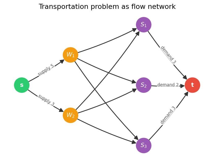
This is a minimum-cost flow problem in disguise. We construct the following network:
- Create a source and a sink .
- For each warehouse , add an arc with capacity and cost .
- For each warehouse and store , add an arc with capacity 1 and cost .
- For each store , add an arc with capacity and cost .
A minimum-cost maximum flow in this network pushes exactly units from to (saturating all supply and meeting all demand) at minimum shipping cost. The flow on arc tells us how many units to ship from warehouse to store .
Consider a small example. Two warehouses supply and units. Three stores demand , , and units. The shipping costs are:
| Store 1 | Store 2 | Store 3 | |
|---|---|---|---|
| Warehouse 1 | |||
| Warehouse 2 |
The minimum-cost flow routes the goods along the cheapest paths: warehouse sends units to store (cost ) and units to store (cost ), warehouse sends units to store (cost ) and unit to store (cost ). Total cost: . The successive shortest paths algorithm from Part 6 would find this solution automatically.
The Assignment Problem
A special case of the transportation problem arises when every supply and every demand is exactly : we have agents and tasks, and each agent must be assigned to exactly one task. The cost of assigning agent to task is , and we want to minimize the total cost.
Definition 15. The assignment problem asks for a minimum-cost perfect matching between agents and tasks, given a cost matrix .
This is equivalent to finding a minimum-cost maximum flow in a bipartite network with unit capacities — combining the bipartite matching reduction from Part 5 with the cost dimension from Part 6.
The assignment problem has a rich history and a famous dedicated algorithm: the Hungarian method, developed by Harold Kuhn in 1955 (based on earlier work by Hungarian mathematicians Dénes König and Jenő Egerváry). The Hungarian method runs in time, which is faster than applying a general min-cost flow algorithm. But conceptually, it can be understood as a specialized version of the successive shortest paths algorithm applied to a bipartite network with unit capacities2.
Minimum-Weight Bipartite Matching
The assignment problem assumed equal numbers of agents and tasks and required a perfect matching. But we can also ask: given a bipartite graph with edge weights, find a maximum matching of minimum total weight. This is the minimum-weight bipartite matching problem.
The reduction to minimum-cost flow is almost identical to the assignment problem. We build a bipartite flow network with unit capacities (as in Part 5) and assign cost to each arc from to . Arcs from and to get cost . A minimum-cost maximum flow then gives a maximum matching of minimum weight.
This generalizes our work on bipartite matchings from the graph theory series. In Part 8 of that series and Part 5 of this series, we found maximum matchings without caring about edge weights. Now, with minimum-cost flows, we can optimize over weighted matchings — a strictly more powerful tool.
Shortest Paths
Perhaps the most surprising reduction is that shortest paths — one of the most fundamental problems in graph theory — are a special case of minimum-cost flows.
Given a directed graph with arc costs and two vertices and , we want to find a shortest (cheapest) path from to . This is a minimum-cost flow problem where every arc has capacity and we want to send exactly unit of flow from to at minimum cost.
Theorem 10. The shortest-path distance from to equals the minimum cost of sending one unit of flow from to in the network with unit capacities and costs equal to the arc weights.
Proof. A flow of value with integer values (guaranteed by the integrality theorem) must route exactly unit along a single --path. The cost of the flow equals the total weight of that path. Minimizing the cost is therefore equivalent to finding the shortest path.
This might seem like overkill — why use the machinery of minimum-cost flows for shortest paths when Dijkstra's algorithm works perfectly well? The point is not practical but conceptual: it shows that minimum-cost flows sit at the top of a hierarchy of problems, with shortest paths as a special case.
The Network Flow Hierarchy
Let's step back and see how all the problems we've studied relate to each other. Each problem in the list below is a special case of the one above it:
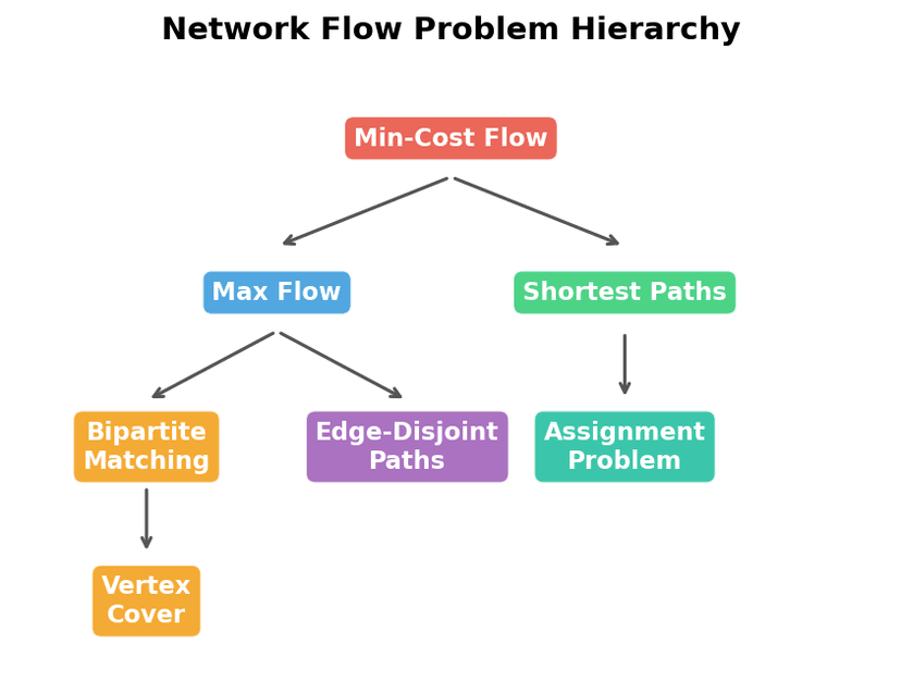
Minimum-Cost Flow — the most general problem: find a flow that maximizes value and minimizes cost.
(set all costs to zero)
Maximum Flow — find a flow of maximum value, ignoring costs.
(unit capacities, bipartite structure)
Bipartite Matching — find a maximum set of disjoint edges in a bipartite graph.
(add edge weights)
Minimum-Weight Bipartite Matching — find a maximum matching of minimum weight (uses min-cost flow).
Meanwhile, from a different angle:
Minimum-Cost Flow (send exactly unit) Shortest Paths
Maximum Flow (unit capacities) Edge-Disjoint Paths (Menger's theorem)
And the Max-Flow Min-Cut Theorem connects maximum flow to minimum cuts, while König's theorem connects bipartite matching to vertex covers. All of these dualities are instances of the same underlying principle: LP duality applied to network structures.
This hierarchy explains why network flow theory is so central to combinatorial optimization. By solving one general problem — minimum-cost flow — we can solve shortest paths, maximum matchings, transportation problems, assignment problems, and many more, all as special cases.
Wrapping Up the Series
We've come a long way since Part 1's supply chain motivation. Let's trace the journey:
Part 1 introduced network flows as a tool for real-world optimization. Part 2 laid the formal foundations with flow networks, flows, cuts, and weak duality. Part 3 proved the Max-Flow Min-Cut Theorem using residual graphs and augmenting paths. Part 4 turned theory into practice with the Ford-Fulkerson method and the Edmonds-Karp algorithm. Part 5 demonstrated the versatility of maximum flow through applications to bipartite matching, edge-disjoint paths, and project selection. Part 6 introduced costs, the negative cycle optimality condition, and algorithms for minimum-cost flows. And here in Part 7, we saw how minimum-cost flows unify a wide range of classical problems.
Throughout, we've seen a recurring theme: the interplay between primal objects (flows, matchings, paths) and dual objects (cuts, covers, bottlenecks). This duality — the idea that the best solution to one problem is always certified by the best solution to a related problem — is one of the deepest and most useful principles in all of optimization.
If you've followed both this series and the Introduction to Graph Theory, you now have a solid foundation in the combinatorial structures that underpin much of theoretical computer science and operations research. From Euler's bridges to minimum-cost flows, the journey has been one of increasing abstraction and power — and there is always more to explore.
Footnotes
We can also use capacity on the arcs from warehouses to stores without changing the problem, since the supply and demand constraints already limit the flow. ↩
In the successive shortest paths framework, each augmentation matches one agent to one task along the cheapest augmenting path. After augmentations, all agents are matched. The potential-based Dijkstra approach yields exactly the Hungarian method. ↩